The Details of a Ballistics Calculator Solver

The increasing popularity of long range rifle shooting has shooters investigating ballistics calculators. Particularly popular are various apps designed to run on smart phones. But what is the difference between them all? Are they all the same, or are some better than others?

In this article, I want to address one particular part of the ballistic calculator - the methods used to calculate the trajectory. I won't get into differences in bullet libraries, user interfaces, or anything of that sort, because that is largely a matter of user preference.

There are lots of online forum discussions about which solver works best and which is most accurate. They seem to go on and on, back and forth, with little agreement. Why is that? Because it does not matter! Unless you are writing the software yourself, there is no practical difference, although there is a clearly favored method. More on this in a bit.

What the Heck is a DOF?

Before I get into two of the more popular methods of solving for ballistics trajectories, lets take a look at some possibly unfamiliar terminology - the Degree Of Freedom, otherwise known as DOF.

What exactly does that mean? In the context of the physics of moving objects, a rigid object like a bullet has 6 degrees of freedom. That is, it can move in 6 different ways. It can move linearly (translate) in the x, y, or z directions, and it can rotate about the x, y, and z axes.

In other words, the location and orientation of a bullet can be fully described by six numbers. That's it. That's all it means.

The Equations of Motion

When coming up with a ballistics model, we have to start with the fundamentals of physics. In this case, we go all the way back to Isaac Newton and his laws of motion. Most notably,

F = ma

If we consider all of the forces that act on a bullet, and we know its mass, we can determine its acceleration at any given point in time. With that, we can determine its position and speed at any point in time, which is really what we're after.

But how do we combine all those forces into an equation we can solve? It's tricky, but you wind up with a coupled system of differential equations. Solving those differential equations together results in more (regular, every day) equations that we can use directly to calculate a specific numerical trajectory based on our inputs. This is known as an analytical solution to the equations of motion.

6DOF - The Kitchen Sink

The 6DOF method accounts for all (non-negligible) forces acting on a bullet, and requires solution of a system of six differential equations to get an answer - one for each DOF.

The up side to this is that you get a trajectory that fully accounts for the physics. Effects due to bullet yaw and spin are modeled and you will see things like spin drift, epicyclic swerve, aerodynamic jump, and more. It all gets calculated directly from the basic physics.

The trouble is that in order to do that, you need a couple dozen (depending how you count) separate aerodynamic coefficients and other inputs, some of which vary with velocity and/or yaw. For each bullet. You also must know the specific starting conditions for the bullet travel, which is not quite as simple as just knowing the muzzle velocity.

And it gets worse. These coefficients are not as easily measured as the BC that you're familiar with. Many of them display non-linear behaviors that further complicate the math. But without this data, the model is useless.

Unfortunately, there are only a few bullets for which we can access this data - a handful of military projectiles - not exactly the stuff that we shoot in competition.

Bottom line: the 6DOF method is great, but utterly impractical. It's of no use to us as sportsmen. It is very useful in military applications such as high angle artillery fire, rockets, or machine gun fire from moving aircraft. The military has collected the data they need for these applications and can make use of the 6DOF model when it is called for. We're out of luck.

However, all is not lost. It turns out the rotational effects can be ignored and you can still calculate a useful, accurate trajectory for our purposes. Even better is that there are ways of adding the important rotational effects back in without resorting to a full blown 6DOF model.

UPDATE (12/23/2016): Lapua has recently released a 6DOF program aimed at sportsmen that uses 6DOF data for a selection of their bullets, so I will eat some crow on this. "No use to sportsmen" is is simply not the case anymore. It's unclear how exactly Lapua went about getting at all the data they needed (whether the data was calculated or measured, for example), but they did a lot of work one way another to provide what is currently the most sophisticated ballistics solver on the market (and it's free - can't complain about that). I will keep an eye on it as it develops. Perhaps a review is in order.

3DOF - The Point Mass Method

The 3DOF method is exactly what it sounds like - it accounts for only three of the six degrees of freedom. More specifically, it ignores the three rotational degrees of freedom and deals only with the three translational ones. In other words, it ignores yaw and spin. Because of this, the name "Point Mass" is used - the projectile is modeled as a point in space.

Because of this simplifying assumption, we can greatly reduce the complexity of the equations of motion. We go from six differential equations down to three. More importantly, we get rid of all of the aerodynamic coefficients needed except one - the drag coefficient, which varies (greatly) with velocity.

So the 3DOF model gives us greatly enhanced usability at only a slight cost in fidelity. It will fail significantly to predict mortar fire, but it does very well with small arms.

The Drag Problem

Remember when I said that what we want is an analytical solution to the equations of motion? Well it turns out you can't get one. It's too difficult. That elusive formula where you can plug in velocity, BC and some other data and have it spit out an exact solution to the 3DOF or 6DOF equations of motion? It doesn't exist.

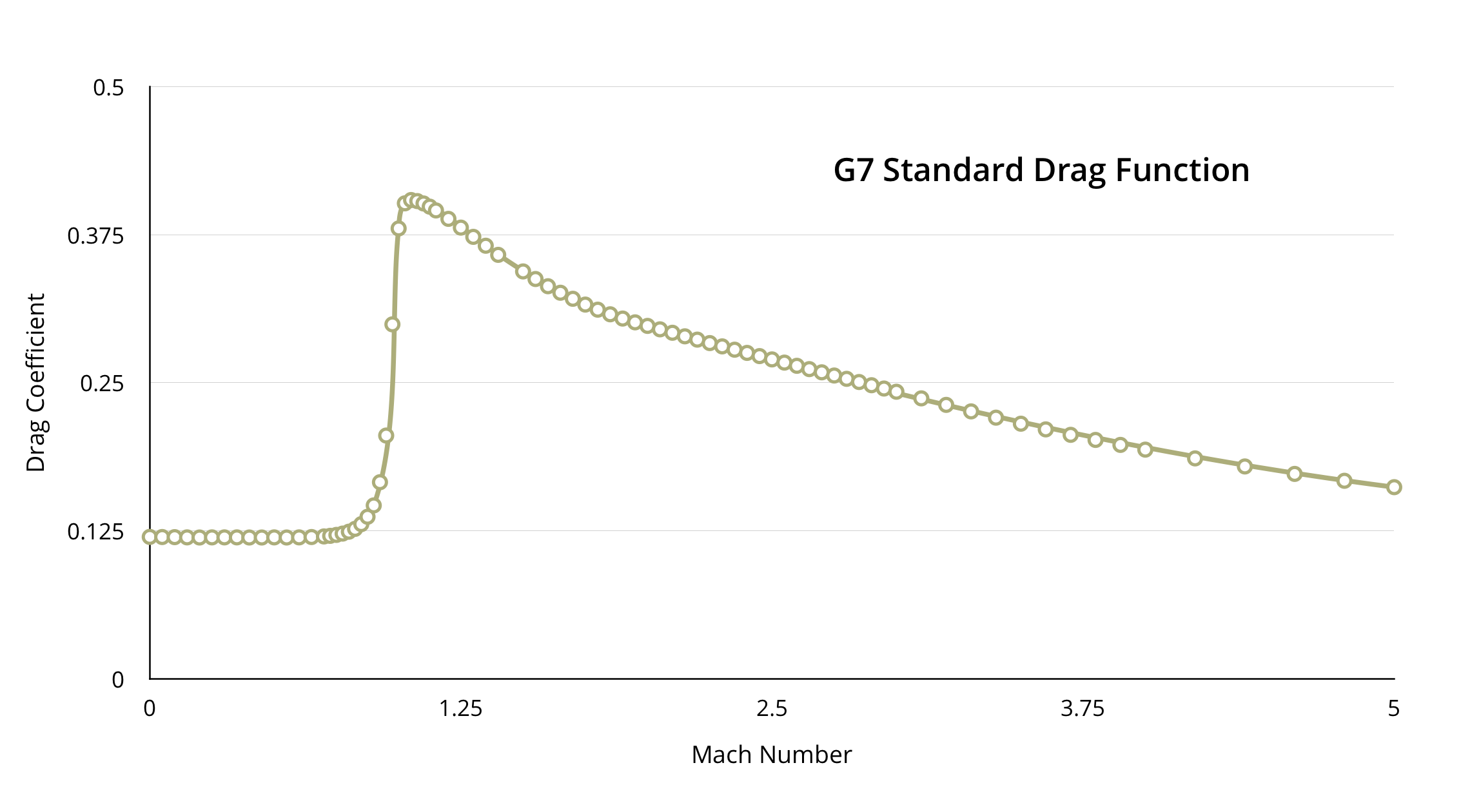
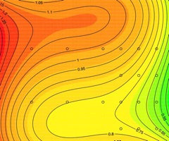
The reason for this is that drag is not a simple thing that follows simple equations. The other forces required by the 6DOF model are similarly complex, but we'll just concern ourselves with drag for the moment because that's all we need for Point Mass. The drag on a bullet is varies smoothly both below and above the speed of sound. But in the region near Mach 1.0 (the speed of sound in air), all bets are off and it the drag changes dramatically. The exact shape of the curve is different for every bullet but they all look vaguely like this one, which is known as the G7 standard drag curve.

So if there is no simple, solvable equation to accurately model a bullet's drag curve, what do we do? Back in the day, people cheated. They came up with simplifying assumptions. For example, if you assume drag follows a simple equations closely enough, and that the angle of fire is small, you can simplify things down to the point where you can solve the equations of motion and get your analytical solution. But you'll have introduced some error with those simplifications.

The Siacci method is a method that accounts for more realistic drag, but still retains the small angle of fire assumptions. It's very clever, mathematically speaking, and it was used by the US military until the 1940s and even longer by the civilian market. It's kind of a pain, and involves some significant compromises, but it provides pretty good accuracy for something developed in the late 1800's.

Dr. Arthur Pejsa's famous Pejsa method is a similarly clever method that allows for the equations of motion to be solved by simplifying them - he approximated the drag with some simple equations and came up with a method that is almost as good as what we use today, but that only requires high school math. That's a great achievement, and his method is far simpler than Siacci's, but it's still not perfect.

Numerical Methods

The development of digital computers during World War II made it possible to solve the complete 3DOF and 6DOF equations, while using any arbitrary functions (curves) for drag, and in the case of the 6DOF model, the other aerodynamic coefficients. Simplifying assumptions like low angles of fire and approximate drag curves were no longer necessary. 6DOF still requires massive efforts in data collection, but 3DOF does not, and thus became very widely used. Bob McCoy referred to it as "the backbone of modern exterior ballistics".

In fact, the point-mass trajectory approximation is so generally useful, it may well be considered the backbone of modern exterior ballistics.

-Bob McCoy

But there's a catch. Instead of analytical solutions we must find numerical solutions. That's a fancy way of saying that we can approximate the results of the analytical solution for a specific set of numerical inputs. But in doing so, we introduce some error along the way - you can think of it as sort of like a rounding error. The full physics of the model are accounted for in the equations, but the solution itself has introduced error.

The way numerical solutions work is that you step along the trajectory, calculating in tiny steps as you go. Each step uses the results of the last step. It turns out that that "rounding" error can be reduced by stepping along the trajectory in smaller increments. The more steps you take, the less error you introduce. (Mathematicians, please don't call me out on this - I know it's a bit of an oversimplification, but I'm trying to keep things easy here.) Since computers are doing all the work, we can effortlessly take a lot of steps and get a very accurate solution.

For example, a common technique is to step through time. That means you might calculate the trajectory for every 0.001 seconds of bullet flight. That might be 1,500 separate calculations along the flight path to 1,000 yards. No sweat for a computer. You can also step along distance - it's often convenient to step every foot or yard thought the trajectory. Either way, very low errors can be achieved.

Every Point Mass solver solves the same equations, but they might do it differently. There are many, many numerical techniques for solving differential equations. That's one reason you see slightly different results from different Point Mass calculators.

To illustrate, I'll compare three free solvers you can find on the web. The Applied Ballistics calculator steps through time. JBM uses a fairly sophisticated algorithm to determine the optimal step size dynamically, increasing the calculation speed (not that it matters much). The Bison Ballistics calculator steps through distance. All three solvers are based on the equations described in Bob McCoy's (and other) books, but all three yield slightly different results with the same inputs.

So how does this numerical method get us around the drag problem? It allows us to measure drag (for example, with a wind tunnel, spark range, or doppler radar), and tabulate it as a function of drag coefficient vs Mach number. Since at any given tiny calculation step, we will know the precise Mach number, we can just look up the corresponding drag coefficient. It's just a table of numbers, so there is no need to calculate anything. The better we measure drag (and Doppler does it very well), the more accurately we can calculate a solution.

So to recap, there are two areas in which we simplify the equations of motion. First, when we go from 6DOF to 3DOF. Then, when we solve the 3DOF equations. Some (obsolete) methods choose to simplify the equations of motion and tolerate the (sometimes significant) errors introduced by those simplifications, while the Point Mass method opts to keep the equations of motion intact, accepting that there will be some small error introduced in the numerical solution. The Point Mass method is preferable because it allows for very accurate drag data to be used in the calculations.

Solving Is Solved

Now here's the part I told you I'd get to. None of that matters. This is very important to understand. The physics of ballistics have been known and understood for roughly a century. We knew the equations of motion for projectiles long before we had practical ways of solving them. This is well trodden aerospace engineering and has been the basis of all manner of flight technology. This is not up for debate.

Likewise, with access to modern computers, solving the equations of motion has become a trivial act, achievable by any undergraduate engineering student. I wrote the Bison Ballistics calculator from scratch in my spare time over a period of two weeks. Any competent aerospace engineer could do the same with a copy of Bob McCoy's book. JBM Ballistics has some C code on their website free for anyone to download and modify.

As long as the person writing the code knows what they are doing and the code is free of bugs, any of the various commonly used methods will work. However, every serious engineer that I know of uses the Point Mass method or an extension of it. The Point Mass method is not proprietary - it's an application of basic physics in a standard way that was developed largely by the US military over the last 100 years. It's not going anywhere, and it works.

Our new, simplified formulas and method are nearly as accurate as these much more complex methods for the shallow trajectories considered herein.

-Arthur Pejsa

Several smart people have come up with alternate ways at solving the ballistics equations, often attempting to model drag with equations (as opposed to the empirical standard drag curves or Doppler based curves). That is interesting to me in an academic sort of way, and they do work pretty well (within thier constraints). But they're just not necessary these days. I would include the work of Arthur Pejsa and the lesser known George Klimi (who strangely uses Snell's Law in his calculations) in this category. Interesting, but largely academic stuff.

A Note about Ballistic Coefficients

You'll notice that I've been using the term drag coefficient (Cd) rather than the commonly used ballistic coefficient (BC). They are not the same thing. The underlying math of the Point Mass method uses Cd to calculate the trajectory. Cd is a standard engineering term used throughout the profession. Ideally we would have a table of Cd vs Mach number for every bullet. Practically, this is very difficult to get. Lapua is the only manufacturer who currently provides this data, which is derived from their Doppler radar testing. This appears to be changing, as Hornady recently has made some noise about their Doppler capabilities. I hope this marks the beginning of a change industry wide.

In the absence of perfect Cd vs Mach data for your specific bullet, we can use standard drag functions, like the G1 and G7 curves we hear so much about. But in order to use those (which are known drag curves for very specific standard projectiles) with your actual bullets, we have to scale them with a BC. The end result is a drag table that almost fits your bullet. Some will be a better fit with a scaled G1. Most will be a better fit with a scaled G7. Neither will be as good as a Doppler-derived Cd vs Mach table that requires no BC at all.

Data is Difficult

So why all the disagreement about which solver is better? I believe the main reason is that no matter the solver, you have the Garbage In Garbage Out (GIGO) problem. No matter how careful they are, people are going to unknowingly enter data that's just a little bit wrong, and the calculator results don't match the real life bullet impacts. This leads to confusion. Is it the calculator? Is it the data?

In my experience, people are a lot more confident in their data than they ought to be, and tend to blame the calculator, which in all fairness will be a little off for reasons I've already discussed. But when your BC is 5% off, your velocity is 2% off, your scope clicks are 1% off, and your range is 3% off, you will get a significant error at long range that you can't blame on the calculator. That's on you. But people do, and so they look for a better calculator. Don't do that. It's a fool's errand. Don't succumb to overconfidence bias.

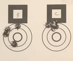
Worse still, they give up and try to true their results to what they see on paper. A little tweak is ok. A little. There are smart ways of doing that and there are not so smart ways of doing it. The most common, and least intelligent way, is to just start randomly fudging numbers until the calculator tells you what you want it to. You will probably get even worse results at other ranges, and now you're screwed because your numbers don't match any physical reality. The best way to "true" your calculator is to accurately measure all of the inputs. If you're still off, it won't be by much, and the culprit will likely be the BC. This is a topic unto itself, so I'll just leave it at that for now.

Another reason for debate is that there are a handful of proprietary solvers on the market who's creators do not explain how they work in any detail. While this is understandable from a business point of view, all calculators that make use of something as simple as a BC to get to a result will be taking some short cuts along the way. So it's tough to broadly evaluate the strengths and weaknesses of proprietary calculators. Since we're dealing with black boxes, we can only evaluate the output, which is difficult to do in a comprehensive manner. So this also opens the door for debate.

And while proprietary calculators might have some interesting features that appeal to their users, it's my opinion that it is not possible to materially improve on Point Mass without adding additional data (such as rotational effects). The combination of Point Mass and Doppler-derived drag tables is very accurate, and has been the cornerstone of the aerospace industry's ballistics technology for quite some time.

Damon Cali is the creator of the Bison Ballistics website and a high power rifle shooter currently living in Nebraska.